Lecture 10: Signals and Audio

HTML Slides  │ PDF Slides  │ Demo code on GitHub

Topic overview#

• Introduction to signals
• Audio as a 1D signal
• File formats
• A brief intro to signal processing

Resources used:

• Various textbooks from my undergrad
• DSPguide.com seems like a pretty good resource

What is a signal?#

“A [continuous/discrete] signal is a function of independent variables that range over [a continuum/discrete] values” - Jerry L. Prince, Medical Imaging Signals and Systems

• Common notation: $x(t)$ for continuous, $x[n]$ for discrete
• Signals are discretized by sampling at some fixed interval $dt$
• The sampling rate is informed by the frequency content of the data: $$f_s \ge 2 f_{max}$$ (but in practice is much higher)

Frequency content of a signal#

• A discrete time domain signal can be represented as: $$x[n] = \sum_{k=0}^{N-1}\left[a_k\cos\left(\frac{2\pi k n}{N}\right) + b_k\sin\left(\frac{2\pi k n}{N}\right)\right]$$
• Or, using Euler’s formula $e^{j\theta} = \cos\theta + j\sin\theta$: $$x[n] = \sum_{k=0}^{N-1}c_k e^{j\frac{2\pi k n}{N}}$$ where the complex coefficients $c_k = a_k + jb_k$ and $j = \sqrt{-1}$

Fourier Transform#

• To figure out what the coefficients $c_k$ are, we can use the Discrete Fourier Transform (DFT): $$X[k] = \sum_{n=0}^{N-1}x[n]e^{-j2\pi \frac{k}{N} n}$$ where each element of $X[k]$ is the coefficient $c_k$ for frequency $k$
• This can also be inverted to get back the original signal: $$x[n] = \frac{1}{N}\sum_{k=0}^{N-1}X[k]e^{j2\pi \frac{k}{N} n}$$

Where we left off on March 17#

Symmetry in the frequency domain#

• Since a real-valued signal in time is composed of both sine and cosine components, its DFT has conjugate symmetry $$X[N-k] = X[k]^$$ where $^$ denotes the complex conjugate
• This means the negative-frequency half of the spectrum is redundant
• In practice, for real-valued data, we often only inspect:
  • magnitude: $|X[k]|$ to see “how much” of each frequency is present
  • phase: $\angle X[k]$ to see alignment/shift information

Frequency vs Time Domains#

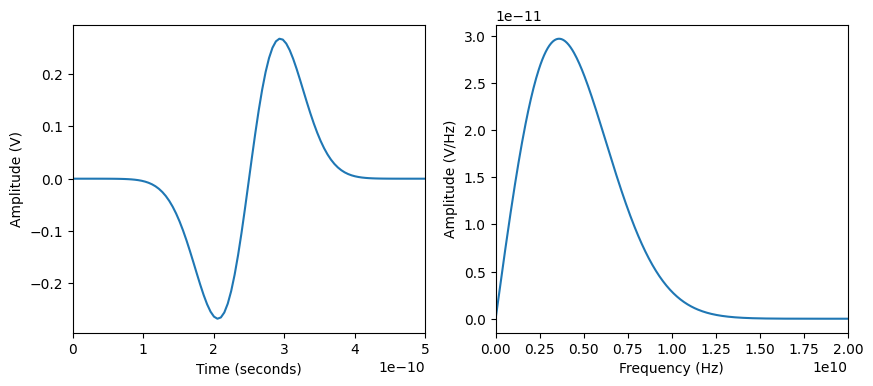
• $f = \frac{1}{t} \implies$ short time = high frequency, small frequency = long time

Example signal: Audio#

• Once you think of a signal as being a weighted sum of frequency components, you can do some fun things with it
• We can extract information, downsample, remove noise, etc
• Example: a typical .wav file
  • Uncompressed
  • 16 bits per sample (bit depth)
  • 48 kHz sampling rate
  • mono (1 channel) or stereo (2 channels)

What about .mp3? .ogg? I would use ffmpeg to convert to .wav

Preparing data#

• Assuming we’re starting with a collection of audio files, we can either:
  • Extract features and save as tabular data
  • Use the raw audio signal as input
• We can preprocess and store the data, or preprocess on the fly

What considerations might go into this decision? What should always be stored regardless of the approach?

Preparing audio data#

• Data for learning tasks is easiest to work with if it is consistent
• For audio signals, this could include:
  • Decompressing and converting to .wav
  • Downsampling
  • Aligning and cropping primary signal
  • Converting to mono/stereo
  • Extracting features
• librosa can help with this (and can apparently handle mp3 too!)

Coming up next#

• 2D signals (aka images)
• Strategies and software for labelling data

By next week you should have some idea of what kind of dataset you want to curate and label for Assignment 3