Lecture 5: Numeric transformations
HTML Slides
 │ PDF Slides
 │ Demo code on GitHub

Topic overview#
- Why transformations are necessary
- Common transformations
- Dimensionality reduction
Resources used:
- Feature Engineering Chapter 6
- Hands on Machine Learning with Scikit-Learn and Tensorflow/PyTorch, Chapter 4. Available at MRU Library
- Scikit-learn user guide: Chapter 7
- Introduction to Machine Learning with Python. Available at MRU Library
Common 1:1 transformations#
“Most models work best when each feature (and in regression also the target) is loosely Gaussian distributed” – Introduction to Machine Learning with Python
- Scaling: normalization or standardization
- Nonlinear transforms: log, square root, polynomial
- Fancier methods: Box-Cox, Yeo-Johnson
A brief intro to gradient descent#
Many linear models minimize some cost function through gradient descent
The gradient is a vector of partial derivatives $$\nabla f = \begin{bmatrix} \frac{\partial f}{\partial x_1} \ \frac{\partial f}{\partial x_2} \ \vdots \ \frac{\partial f}{\partial x_n} \end{bmatrix}$$
for some scalar-valued $f(\mathbf{x})$
Descending the gradient#
For a loss (or cost) function such as $MSE(\mathrm{\theta}) = \frac{1}{m}(\mathbf{X}\mathbf{\theta} - \mathbf{y})^T(\mathbf{X}\mathbf{\theta} - \mathbf{y})$
Start with a random $\mathbf{\theta}$
Calculate the gradient $\nabla_{\mathbf{\theta}}$ for the current $\mathbf{\theta}$
Update $\mathbf{\theta}$ as $\mathbf{\theta} = \mathbf{\theta} - \eta \nabla_{\mathbf{\theta}}$
Repeat 2-3 until some stopping criterion is met
where $\eta$ is the learning rate, or the size of step to take in the direction opposite the gradient.
Visualizing in 2D#
- The gradient has $m + 1$ dimensions, where $m$ is the number of features
- step size $\eta$ is a scalar parameter
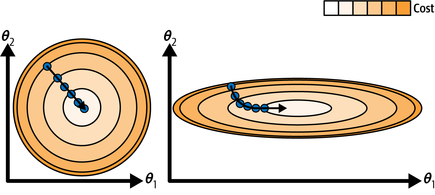
Main takeaway: feature should be more or less on the same scale
Approaches to scaling#
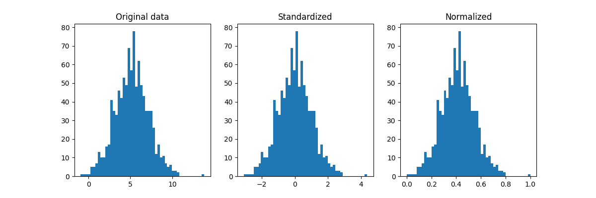
Standardize: $x_{scaled} = \dfrac{x - \mu_x}{\sigma_x}$
Normalize: $x_{scaled} = \dfrac{x - \mathrm{min}(x)}{\mathrm{max}(x) - \mathrm{min}(x)}$
Nonlinear transforms#
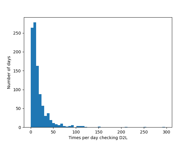
- Common case: count data
- Example: Ask 1000 students how often they checked D2L that day
- Not a Gaussian distribution!
- What about the central limit theorem?
Where we left off on January 27#
Transformations in training vs inference#
- Define functions, e.g.
def standardize(X, mu, sigma): return (X - mu) / sigma - Compute scaling parameters on the training data, then stash them somewhere:
mu = X_train.mean()
sigma = X_train.std()
# ... later on, during inference
X = standardize(X, mu, sigma)
What would happen if
standardizeinstead computed values on the fly? What else am I missing here?
Manual approach in the wild#
You may run across magic numbers, e.g from the PyTorch tutorials:
import torch
from torchvision import transforms, datasets

data_transform = transforms.Compose([
        transforms.RandomResizedCrop(224),
        transforms.RandomHorizontalFlip(),
        transforms.ToTensor(),
        transforms.Normalize(mean=[0.485, 0.456, 0.406],
                             std=[0.229, 0.224, 0.225])
    ])
This really should have a comment! Derived from ImageNet.
An alternative solution: Scikit-learn Pipelines#
- Hard-coding scaling (and other) parameters is okay, provided you can justify the choice and document where they came from
- Scikit-learn has a handy Pipeline class that handles this for you
- Each step in the pipeline has a
fitandtransformmethodfitcomputes parameters from the training datatransformapplies the transformationfit_transformdoes both – only use on training data!
- You can call these functions on the whole pipeline to fit or apply all in one go
Pipeline#
- The Pipeline class chains things together in a linear fashion
- Output from one step is input to the next
make_pipelineis slightly simpler syntax (no names needed)from sklearn.pipeline import make_pipeline, Pipeline pipeline = make_pipeline( StandardScaler(), SGDClassifier() ) # or, equivalently: pipeline = Pipeline([ ('scaler', StandardScaler()), ('sgd', SGDClassifier()) ])
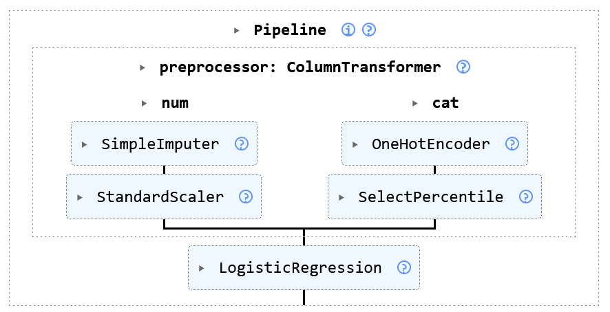
ColumnTransformer#
- The ColumnTransformer selects specific features and processes in parallel
- Most of the time mixed dataset need this
1:many transformations#
- So far our numeric transformations have been 1:1
- 1:many creates multiple features from 1, like binning
- Basis expansion introduces nonlinearity to a continuous feature, e.g.: $$x \rightarrow [\beta_1x, \beta_2x^2, \beta_3x^3]$$
- More exciting is the spline version where you can define different polynomials for different ranges of $x$
Where we left off on January 29#
Dimensionality reduction methods#
many:many transformations#

- Linear projection methods create new features: $$X^* = XA$$ where $A$ is the projection matrix and $X^*$ is the transformed data
- We can use this for dimensionality reduction by only keeping some of $X^*$
- Example: Principle component analysis (PCA) finds the set of orthogonal vectors that explain the most variance
Variance and covariance - Review (?)#
The variance of a single feature $\mathbf{x}$ is: $$\mathrm{var}(\mathbf{x}) = \frac{\sum_1^n (x_i - \mu_x)^2}{n}$$
The covariance between two features $\mathbf{x_1}$ and $\mathbf{x_2}$ is: $$\mathrm{cov}(\mathbf{x_1}, \mathbf{x_2}) = \frac{\sum_1^n (x_{1i} - \mu_{x_1})(x_{2i} - \mu_{x_2})}{n}$$
Independent variables will have low covariance, but low covariance does not necessarily mean independence!
Covariance matrix#
The covariance matrix between all features in a matrix $X$ is: $$\mathrm{cov}(X) = \begin{bmatrix} \mathrm{var}(\mathbf{x_1}) & \mathrm{cov}(\mathbf{x_1}, \mathbf{x_2}) & \cdots & \mathrm{cov}(\mathbf{x_1}, \mathbf{x_m}) \ \mathrm{cov}(\mathbf{x_2}, \mathbf{x_1}) & \mathrm{var}(\mathbf{x_2}) & \cdots & \mathrm{cov}(\mathbf{x_2}, \mathbf{x_m}) \ \vdots & \vdots & \ddots & \vdots \ \mathrm{cov}(\mathbf{x_m}, \mathbf{x_1}) & \mathrm{cov}(\mathbf{x_m}, \mathbf{x_2}) & \cdots & \mathrm{var}(\mathbf{x_m}) \end{bmatrix}$$
Just like regular variance, covariance scales with the data
If you normalize this, you get the correlation matrix
Back to PCA#
- Principle component analysis, proposed in 1901 by Karl Pearson, is a linear projection of multidimensional data onto the axes of maximum variance
- The axes are found by eigendecomposition of the covariance matrix: $$C = Q\Lambda Q^{-1}$$
- The eigenvectors $Q$ form the new orthogonal basis for the covariance matrix $C$, while the eigenvalues $\Lambda$ represent the amount of variance “explained”
- $X^$ can be calculated as: $$X^ = XQ$$
Dimensionality reduction with PCA#
- Sort in order of decreasing eigenvalue (“amount of variance explained”)
- Keep only the first $k$ eigenvectors to form $Q_k$
- Project data onto this smaller basis: $$X^* = XQ_k$$
- Implemented in Scikit-learn by passing
n_componentstoPCA(), e.g.pca = PCA(n_components=2) # just two axes X_reduced = pca.fit_transform(X)
Linear discriminant analysis (LDA)#
- Similar to PCA, but supervised
- Finds basis that maximize class separability
- Number of projection vectors must be
<= min(n_classes - 1, n_features) - Still uses projections and eigenvalues, but adds some statistical magic
- Key assumptions:
- Features are normally distributed within a class
- Classes have identical covariance matrices
- Implemented in Scikit-learn as LinearDiscriminantAnalysis
Other methods#
- It seems crazy, but random projections can work to reduce dimensionality
- Another many:many transformation that has gained popularity in the “Deep Learning era” is the autoencoder
- These are (typically) neural networks that learn a lower-dimensional representation by training the output to match the input
- The “bottleneck” layer in the middle is the reduced representation
- During inference, the model is chopped in half
Pros and cons of dimensionality reduction#
Pros#
- Can improve model by:
- removing noise
- reducing collinearity
- Lower complexity/compute cost
- Can help with visualization
- Can be informative about features
Cons#
- Throwing out information
- Harder to interpret results
- May not actually improve anything
Higher list of pros, but still… don’t do it unless it’s demonstrably beneficial
Summary#
- Numerical data often needs to be transformed to fit model assumptions
- Standardizing (and maybe normalizing) are very common
- Nonlinear transformations can also be beneficial
- Dimensionality reduction can help with model or visualization
- As usual, let the data be your guide
Coming up next#
Assignment 1 - due Friday, ish (Monday is fine, and let me know if you need more than that)- Already passed!Lab: practice with transformation pipelinesAlready passed!- Next topic: Missing data, outliers, and interaction effects