Lecture 2. Basic machine learning models

HTML Slides html │ PDF Slides PDF  │ Demo code on GitHub GitHub

Topic overview#

  • Some common machine learning tasks and models
  • Evaluating model performance
  • Limitations and assumptions

Resources used:

Machine learning#

  • To appropriately process the data, we need to know why we are doing it and what assumptions we’re making
  • Modern machine learning toolkits (such as scikit-learn) are so easy to use, they’re easy to use inappropriately
  • Goal: just enough understanding to use basic models responsibly

Why are we processing data?#

  • No reinforcement learning in this course, sorry

A selection of common models#

Supervised#

  • Linear/logistic regression
  • Decision trees
  • Support vector machines

Unsupervised#

  • K-means clustering
  • Principle component analysis
Source: Müller, A. C., & Guido, S. (2016). Introduction to Machine Learning with Python. O’Reilly Media, Incorporated. Available at MRU Library.

No free lunch#

  • A theory-heavy paper in 1996 showed that there is no one machine learning algorithm that excels in all situations
  • Subsequent work has confirmed this, e.g. a 2018 analysis
  • Tree-based methods, particularly gradient boosted trees tend to outperform other algorithms the most, but still have limitations
  • What does it mean to “outperform”?
Further reading: http://www.feat.engineering/important-concepts#no-free-lunch

Model evaluation: Classification#

  • True positive: predicted positive, label was positive ($TP$) ✔️

  • True negative: predicted negative, label was negative ($TN$) ✔️

  • False positive: predicted positive, label was negative ($FP$) ❌ (type I)

  • False negative: predicted negative, label was positive ($FN$) ❌ (type II)

  • Accuracy is the fraction of correct predictions, given as:

    $$\mathrm{accuracy} = \frac{TP + TN}{TP + TN + FP + FN}$$

Precision and recall#

  • Precision: Out of all the positive predictions, how many were correct? $$\mathrm{precision} = \frac{TP}{TP + FP}$$

  • Recall: Out of all the positive labels, how many were correct? $$\mathrm{recall} = \frac{TP}{TP + FN}$$

  • Specificity: Out of all the negative labels, how many were correct? $$\mathrm{specificity} = \frac{TN}{TN + FP}$$

Confusion matrix#

Predicted PositivePredicted Negative
True PositiveTPFN
True NegativeFPTN
  • The axes might be reversed, but a good predictor will have strong diagonals
  • There’s also the F1 score, or harmonic mean of precision and recall: $$F1 = 2 \cdot \frac{\mathrm{precision} \cdot \mathrm{recall}}{\mathrm{precision} + \mathrm{recall}}$$
Check out the Wikipedia page for more ways of describing the same information

ROC Curves#

  • The receiver operating characteristic curve is a plot of the true positive rate (recall or sensitivity) vs. false positive rate (1 - specificity) as the detection threshold changes

  • The diagonal is the same as random guessing

  • A perfect classifier would hug the top left corner

Fun fact: the name comes from WWII radar operators, where true positives were airplanes and false positives were noise

Classification model: Support Vector Classifier#

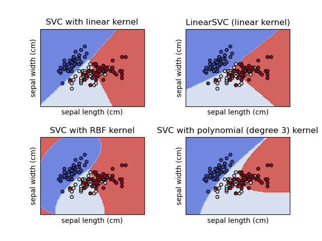
  • Linear model that finds vector(s) to best separate classes
  • “Kernel trick” allows for nonlinear boundaries
  • Check out the SVM Appendix of Hands-on Machine Learning by Aurélien Geron for more info
Image from Scikit-learn documentation

Classification Model: Decision Trees#

  • Family of models including:
    • decision trees
    • random forests
    • gradient boosted decision trees
  • Finds thresholds for features that best separates classes
  • Controllable through depth parameter

Model evaluation: regression#

For a predicted $\hat{\mathbf{y}}$ and actual $\mathbf{y}$, metrics include:

  • Mean squared error: $MSE = \frac{1}{n}\sum_{i=1}^n (y_i - \hat{y}_i)^2$
  • Root mean squared error: $RMSE = \sqrt{MSE}$
  • Mean absolute error: $MAE = \frac{1}{n}\sum_{i=1}^n |y_i - \hat{y}_i|$
  • Mean absolute percentage error: $MAPE = \frac{100}{n}\sum_{i=1}^n \left|\frac{y_i - \hat{y}_i}{y_i}\right|$
  • Coefficient of determination: $R^2 = 1 - \frac{\sum_{i=1}^n (y_i - \hat{y}i)^2}{\sum{i=1}^n (y_i - \bar{y})^2}$ ($R^2$ has some caveats)

Where we left off on January 13#

Regression: ordinary least squares#

  • In 1D, estimate modeled as: $\hat{y_i} = wx_i + b$, where $i$ denotes a sample

  • Vector form: $\mathbf{\hat{y}} = w\mathbf{x} + b$

  • Goal is to minimize the Mean Square Error:

    $$\begin{aligned} MSE &= \frac{1}{m} \sum_{i=1}^m (\hat{y} - y_i)^2 = \frac{1}{m} \sum_{i=1}^m (b + w x_i - y_i)^2\ MSE &= \frac{1}{m} (\hat{\mathbf{y}} - \mathbf{y})^T (\hat{\mathbf{y}} - \mathbf{y}) \end{aligned}$$

Regression: N-dimensional#

  • Most of the time we have $N > 1$ features

  • N-D: $\hat{y_i} = w_1x_{1i} + w_2x_{2i} + … + w_nx_{ni} + b$

  • Common to use a design matrix $\mathbf{X}$ to represent the feature values:

    $$\mathbf{X} = \begin{bmatrix} 1 & x_{11} & x_{12} & \cdots & x_{1n} \ 1 & x_{21} & x_{22} & \cdots & x_{2n} \ \vdots & \vdots & \ddots & \vdots \ 1 & x_{m1} & x_{m2} & \cdots & x_{mn} \end{bmatrix}$$

    where each row is an instance (sample) and each column is a feature.

Regression: N-dimensional#

  • We can rewrite the estimate in matrix notation: $$\hat{\mathbf{y}} = \mathbf{X} \mathbf{\theta}$$

  • The MSE can be written as:

    $$MSE = \frac{1}{m}\sum_{i=1}^m (\hat{y}_i - y_i)^2 = \frac{1}{m} (\mathbf{X} \mathbf{\theta} - \mathbf{y})^T (\mathbf{X} \mathbf{\theta} - \mathbf{y})$$

  • This has a closed form solution, but it is computationally expensive

Regression: Decision trees#

center h:400px

Figure 2-32. Comparison of predictions made by a linear model and predictions made by a regression tree on the RAM price data. Source: Introduction to Machine Learning with Python

Comparison of model families#

Linear models#

  • Very fast, particularly inference
  • Scalable to large number of features
  • Can model nonlinearity with kernel trick
  • Easy to regularize
  • Difficult to interpret
  • Sensitive to parameters and preprocessing
  • Data needs to be on same scale
  • Slow to train on large datasets

Decision Trees#

  • Highly explainable
  • Fast to train
  • Few parameters to tune
  • Little preprocessing needed
  • Provides feature importance
  • Prone to overfitting
  • High variance
  • Poor extrapolation

Coming up next#

  • Exploring and understanding your data
  • Splitting your data
    • Repeatability considerations
    • Stratified sampling
  • Assignment 1: Exploring Calgary traffic data